Report 3 Bangladesh
This report is created based on a publicly available data. The data are available on a Google Sheet. Please see the Data Source section for link. Please note that publicly available data are not official and MAY BE UNRELIABLE. I personally did not verify them. I am using them for educational purposes. Use at your discretion.
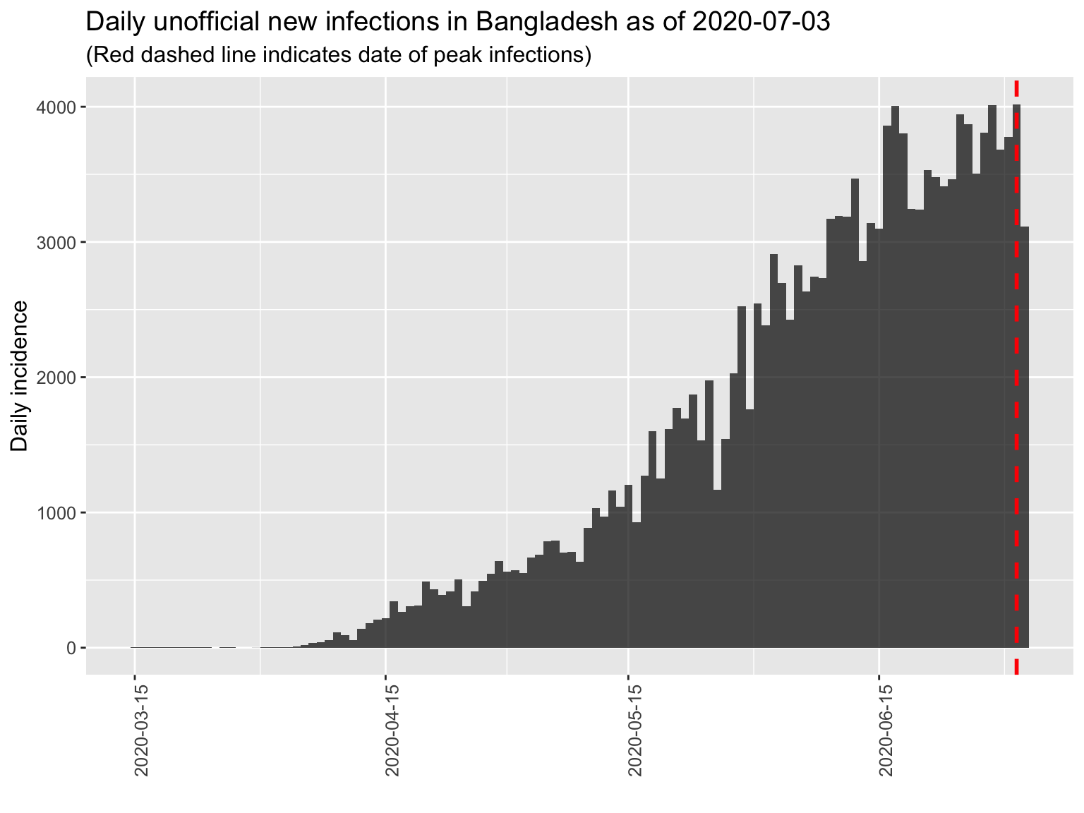
3.1 Epidemic curve and search for peak
The epidemic curve for Bangladesh and a tentative peak. The red line in the plot indicates a potential peak based on available data. IF the peak (red line) is at the far right, then we may not have reached a peak yet. We must have sustained decrease of incidences to be sure about any peak.
We fit a log linear model to estimate the doubling time (growh phase) and halving time (decline phase, when that happens). The estimated fitted line (solid line) with 95% confidence interval (dotten lines) are superimposed on the epidemic curve below.
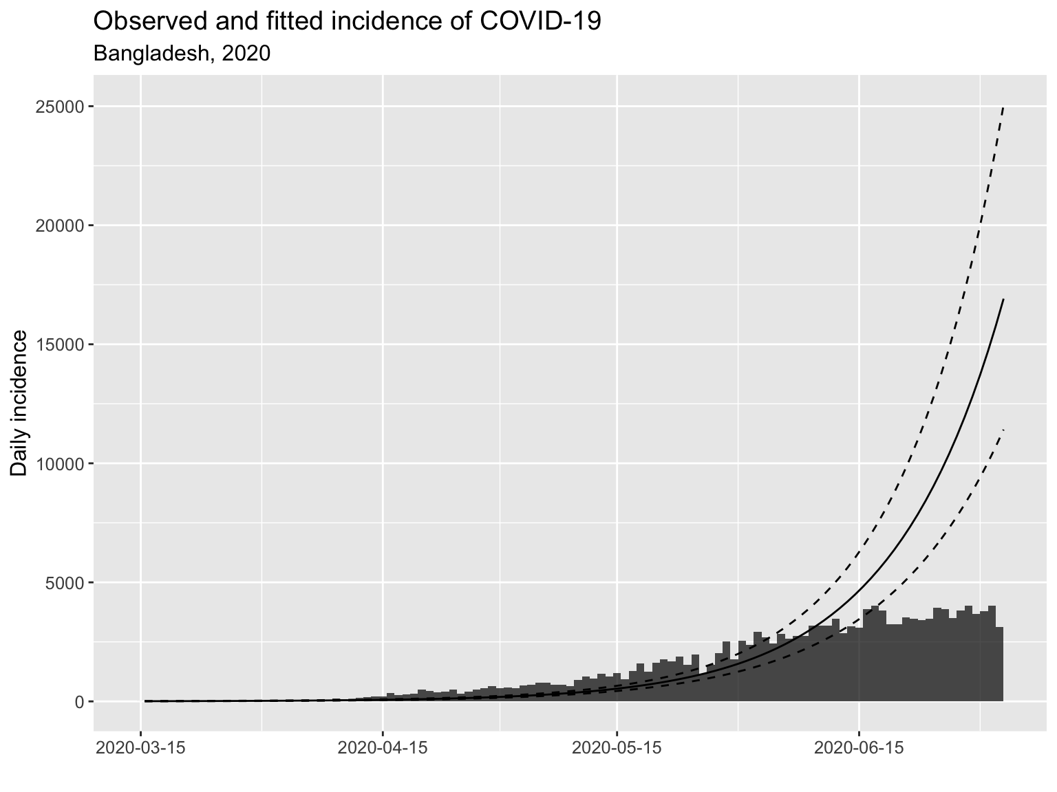
The current doubling time as of 2020-09-10 is 9.9 days with a 95% confidence interval of (9.1, 10.9) days.
3.1.1 Estimating the Overall Reproduction Number, \(R_0\)
The log-linear model estimates the \(R_0\) as follows:
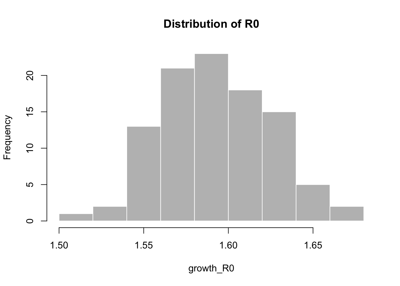
##    Min. 1st Qu.  Median    Mean 3rd Qu.    Max.
##   1.511   1.567   1.591   1.592   1.612   1.679
3.1.2 Estimating the Effectuve Reproduction Number (\(R_e\))
The estimation of effective reproduction number involves the distribution of serial interval (SI). Based on the literature (REF to be added), a gamma distribution with mean 7.5 and standard deviation 3.5
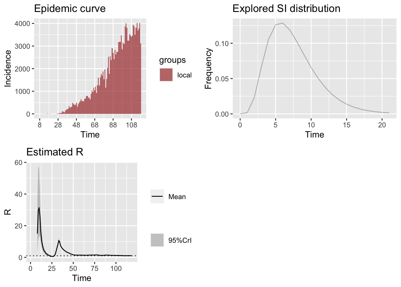
3.1.3 Simulating the \(R_e\) on Weekly Sliding Window
Now we perform a simulation of different SI distribution to obtain the \(R_e\). For this, we vary the parameters of gamma distribution and obtain the following.
# Recalculating with varying SI distribution parameters
# we get these results:

config = make_config(list(mean_si = 7.5, std_mean_si = 3.5,
                                       min_mean_si = 2, max_mean_si =10.0,
                                       std_si = 3.5, std_std_si = 1,
                                       min_std_si = 0.5, max_std_si = 4))
bd_res_uncertain_si <-
  estimate_R(bd_confirmed_cases$daily_cases, method = "uncertain_si",
             config = config)

plot_Ri(bd_res_uncertain_si)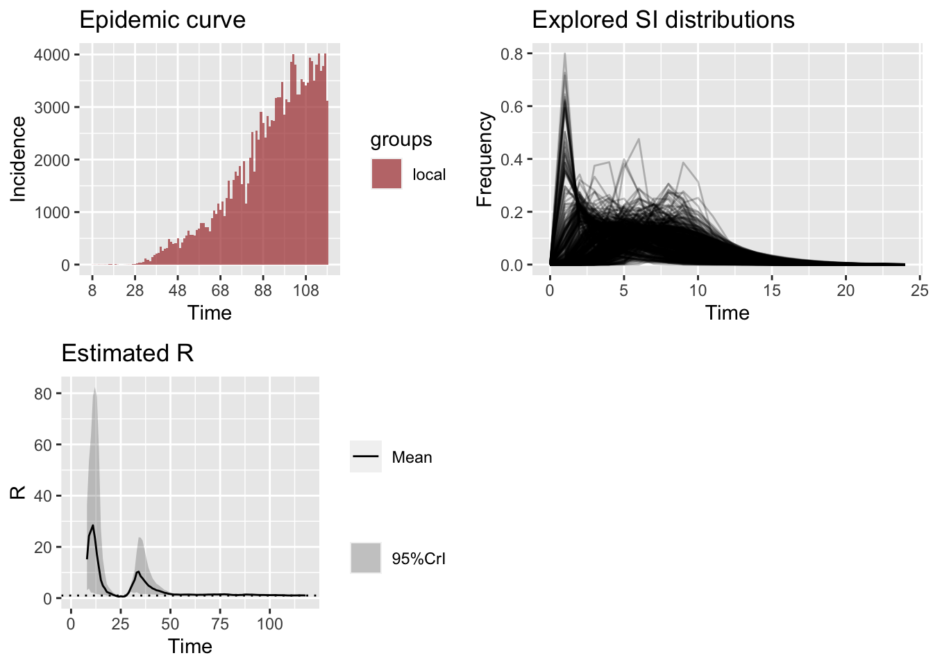
| t_start | t_end | Mean(R) | Std(R) | Quantile.0.025(R) | Quantile.0.975(R) | |
|---|---|---|---|---|---|---|
| 105 | 106 | 112 | 1.046632 | 0.0169938 | 1.0189608 | 1.081899 |
| 106 | 107 | 113 | 1.049673 | 0.0145129 | 1.0231781 | 1.079145 |
| 107 | 108 | 114 | 1.064205 | 0.0138124 | 1.0355469 | 1.090588 |
| 108 | 109 | 115 | 1.067638 | 0.0154839 | 1.0303541 | 1.093207 |
| 109 | 110 | 116 | 1.072344 | 0.0178503 | 1.0300534 | 1.099355 |
| 110 | 111 | 117 | 1.066645 | 0.0202760 | 1.0205370 | 1.096095 |
| 111 | 112 | 118 | 1.027756 | 0.0209605 | 0.9843239 | 1.059694 |
The effective reproduction number based on the last week’s incidences show an average of 1.03 with a 95% confidence interval (0.98, 1.06).
3.1.4 Simulating \(R_e\) on a Monthly Sliding Window
| t_start | t_end | Mean(R) | Std(R) | Quantile.0.025(R) | Quantile.0.975(R) | |
|---|---|---|---|---|---|---|
| 59 | 60 | 89 | 1.328111 | 0.1218987 | 1.093749 | 1.527731 |
| 60 | 61 | 90 | 1.326367 | 0.1225633 | 1.096821 | 1.529301 |
| 61 | 62 | 91 | 1.319118 | 0.1219674 | 1.093018 | 1.523864 |
| 62 | 63 | 92 | 1.312845 | 0.1204491 | 1.092004 | 1.517296 |
| 63 | 64 | 93 | 1.306606 | 0.1180362 | 1.090871 | 1.508910 |
| 64 | 65 | 94 | 1.303426 | 0.1154575 | 1.092073 | 1.502786 |
| 65 | 66 | 95 | 1.296084 | 0.1126439 | 1.088118 | 1.490242 |
| 66 | 67 | 96 | 1.289401 | 0.1097843 | 1.086316 | 1.478005 |
| 67 | 68 | 97 | 1.284089 | 0.1072704 | 1.085707 | 1.467915 |
| 68 | 69 | 98 | 1.268620 | 0.1041213 | 1.075342 | 1.446044 |
| 69 | 70 | 99 | 1.256148 | 0.1003377 | 1.072203 | 1.427868 |
| 70 | 71 | 100 | 1.248356 | 0.0963948 | 1.073534 | 1.414545 |
| 71 | 72 | 101 | 1.247968 | 0.0931521 | 1.078450 | 1.409307 |
| 72 | 73 | 102 | 1.243734 | 0.0904911 | 1.077346 | 1.399898 |
| 73 | 74 | 103 | 1.241699 | 0.0882930 | 1.077199 | 1.392902 |
| 74 | 75 | 104 | 1.224717 | 0.0856263 | 1.063337 | 1.370345 |
| 75 | 76 | 105 | 1.206741 | 0.0819941 | 1.054814 | 1.345852 |
| 76 | 77 | 106 | 1.195827 | 0.0779376 | 1.055362 | 1.329129 |
| 77 | 78 | 107 | 1.182595 | 0.0735190 | 1.051625 | 1.310244 |
| 78 | 79 | 108 | 1.174473 | 0.0690322 | 1.052361 | 1.295629 |
| 79 | 80 | 109 | 1.162138 | 0.0643547 | 1.047242 | 1.275574 |
| 80 | 81 | 110 | 1.168266 | 0.0606673 | 1.060065 | 1.275402 |
| 81 | 82 | 111 | 1.168308 | 0.0584652 | 1.058817 | 1.269725 |
| 82 | 83 | 112 | 1.157930 | 0.0568349 | 1.048442 | 1.254106 |
| 83 | 84 | 113 | 1.146390 | 0.0549897 | 1.041503 | 1.238319 |
| 84 | 85 | 114 | 1.147418 | 0.0532516 | 1.048453 | 1.236274 |
| 85 | 86 | 115 | 1.135368 | 0.0515691 | 1.038929 | 1.221583 |
| 86 | 87 | 116 | 1.127179 | 0.0492675 | 1.037022 | 1.210468 |
| 87 | 88 | 117 | 1.116696 | 0.0464521 | 1.032996 | 1.196648 |
| 88 | 89 | 118 | 1.099904 | 0.0429453 | 1.023926 | 1.175051 |
The effective reproduction number based on the last months’s incidences show an average of 1.1 with a 95% confidence interval (1.02, 1.18).
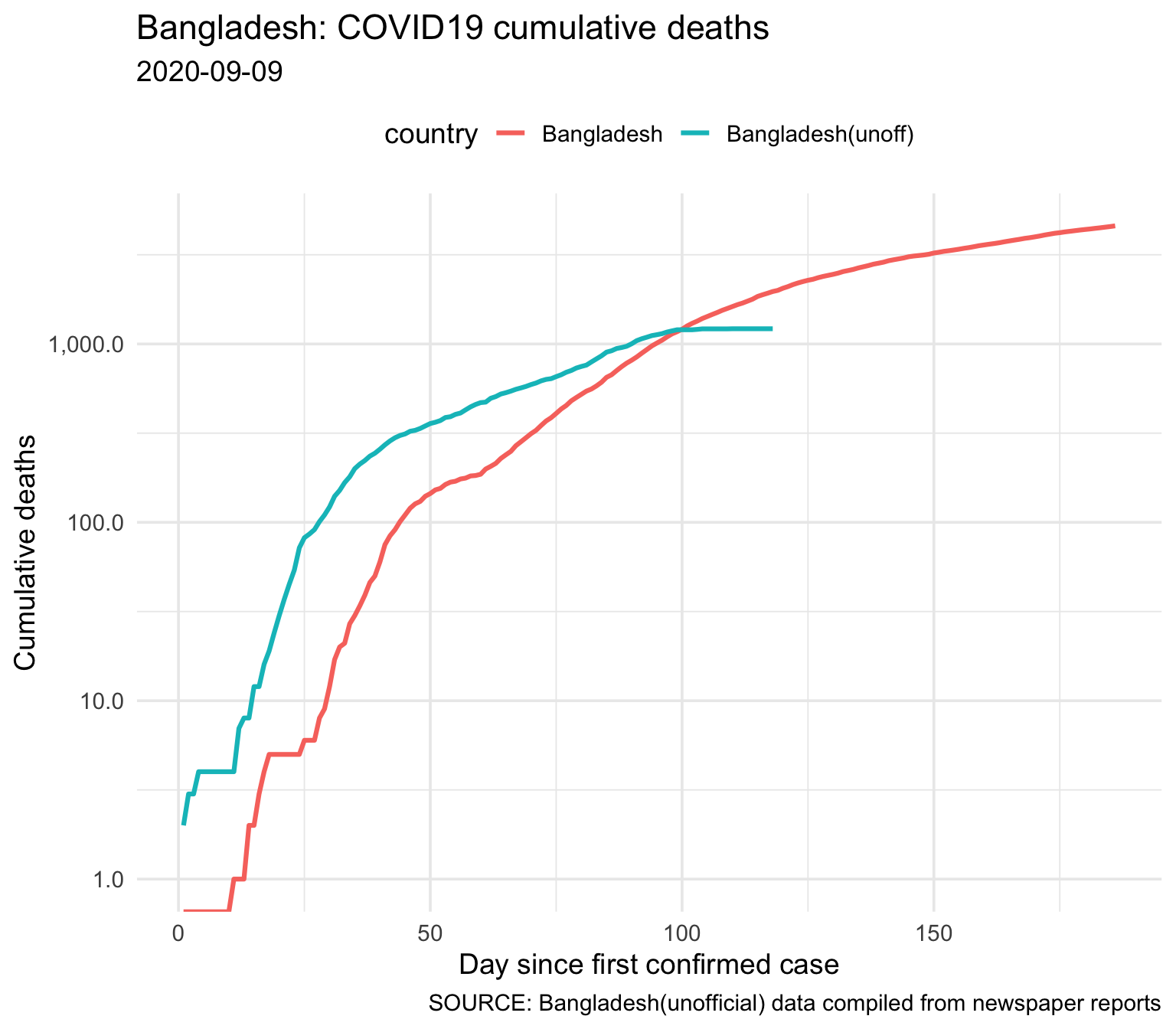
3.1.5 Cumulative Deaths (official and unofficial)
| country | Total Deaths |
|---|---|
| Bangladesh | 4593 |
| Bangladesh(unoff) | 1217 |
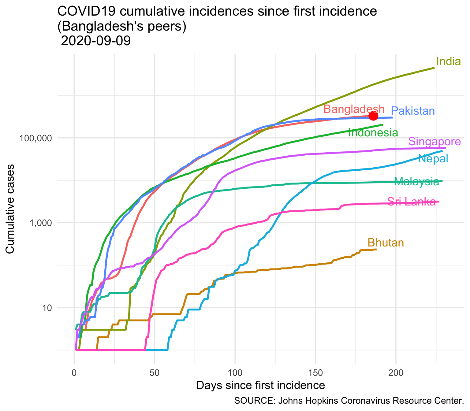
3.2 Bangladesh in South Asia
3.2.1 Infection
| country | Total Cases |
|---|---|
| India | 4465863 |
| Bangladesh | 331078 |
| Pakistan | 300030 |
| Indonesia | 203342 |
| Bangladesh(unoff) | 156391 |
| Singapore | 57166 |
| Nepal | 49219 |
| Malaysia | 9583 |
| Sri Lanka | 3147 |
| Bhutan | 234 |
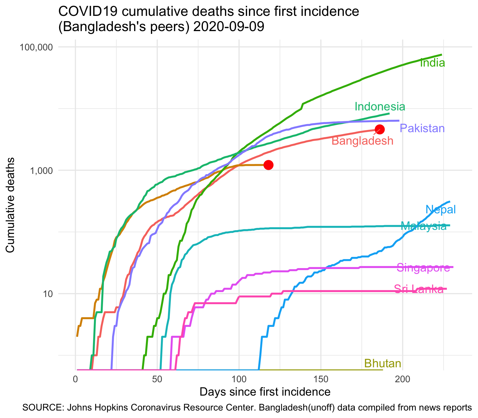
3.2.2 Deaths
| country | Total Deaths |
|---|---|
| India | 75062 |
| Indonesia | 8336 |
| Pakistan | 6365 |
| Bangladesh | 4593 |
| Bangladesh(unoff) | 1217 |
| Nepal | 312 |
| Malaysia | 128 |
| Singapore | 27 |
| Sri Lanka | 12 |
| Bhutan | 0 |
3.2.3 Cases and deaths compared on a specific day
Bangladesh has entered into day 186 since first confirmed case.
| Country | Total cases | Total deaths |
|---|---|---|
| India | 1803695 | 38135 |
| Indonesia | 184268 | 7750 |
| Pakistan | 295053 | 6283 |
| Bangladesh | 331078 | 4593 |
| Malaysia | 8943 | 124 |
| Nepal | 19063 | 49 |
| Singapore | 50369 | 27 |
| Sri Lanka | 2814 | 11 |
| Bhutan | 233 | 0 |